W01 課程介紹
2025-09-10-Wednesday 14:10-17:00 林師模教授 shihmolin@gmail.com (助教Sophia張桂鳳)
| syllabus | phd16-QM(I) | Review of Statistics: Prof.'s: Basic Probability Concepts | 統計自習筆記 |
課本: Principles of Econometrics, 5th Edition | Formulas公式查表 | 課本的學習參考提示與答案 | 筆記: GoogleDoc
工具: p-value | t-critical value |
作業: W03 Asig#1 | W07Asig#2 | WxxAsig#3 |
考試: Exam | Midterm | Final |
同學:11304601劉珮彤, 11304625茉莉(India), (遇Romi同學-說統計很好的-Bisyri Effend想參加2026_LFHintern)
😊喜歡這門課,特地自動重修,這次希望可以盡可能找我們公司或自己感興趣的數據資料做研究。
本週在多倫多,請假!
W02 Review of Statistics
2025-09-17-Tuesday 14:00-17:00 林師模教授
Review of Statistics: Prof.'s: Basic Probability Concepts |
1.問? what's difference betweeen: standardizqtion and nomorlization
2.問? 為何需要standardization?
remove unit
confine the range, in -1<= sd <=1
esay to compare: for the unit has been removed
-注意frequently use公式: var(a+cX) = c^2var(X) 因為 a 是constant 沒有var (coefficient 係數)
-E[(X-EX) (Y-EY)] --> +or- will know the relationship of X and Y, that's call: covarance
雖然X-EX 或但是看不出來strength 這是因為 unit改變就會改變數字。如果想知道strength 強度,可以先做standarlilzation以除去unit。
所以可以用: Measure / SD
公式: Z = (Xi - EX )/S.D.(X)
-Cov(X,Y)=E[(X-EX) (Y-EY)] = {Sumation (X-EX) (Y-EY)} / n
看2,34 Correlation
is a pure number faling between -1 and 1
*注意 要在你的excel加上 增益集-分析工具箱-
這樣你按 資料時 右邊就會出現 「資料分析」這工具。
=自己用lireoffice和Googlesheet 試做個 x體重/y身高 資料表,然後叫他算出 correlation number 相關係數。
這工具還可有其他分析工具,但更複雜的要用Eviews之類軟體來做。
The coverse is not true. 這句話 Why?
Y=a+bX 時 cor = 1
但 如果是個圓的話 cor=0 但 X Y 應該是有關係 but why we got o relationship
因為只能測量 linear relationship 而如果你碰到non-linear relationship時,隨然 cor=0 但是X Y其實是有non-linear relationship的
-2.37
-2.38 記住 weighted sum of rendom variables: 的公式,很重要。常要用到。
問: 為何要sandardization?
答: 因為不可能弄無線多個distribution table, 如果把mean設為0 把sd設為1 那就只要一張table就好了!
probability ditribution table =
見 2.41 只要convaert 原來的Y變成a 做出 Standard normal
2.44 Chi-Square distribution
吸煙與肺癌的研究因為是從兩個獨立的群體(病例與對照)開始,並比較它們的吸煙習慣分布,所以它在統計學上屬於同質性檢驗的應用範疇。
2.46 F statistic distribution (F是偏左的 distribution 都是正的-因都平方, 右邊長尾)
i-learning_2.0
W03 ANOVA: Analysis of variance
2025-09-24-Tuesday 14:00-17:00 林師模教授
★ ■ ▲
wha is the steops of hypothesis
■ Hypothesis testing, ■ANOVA(Analysis of variance) 變異數分析;
ChatGPT說明 The
steps of hypothesis
例如: 100學生數學成績,內有分N M S 北中南三區學生
1.what question? is region -> effect of math score.
2.H0: μ1=μ2=μ3 (μN=μM=μS)
H1: μ1≠μ2≠μ3 either one ≠
3.★ select Test Statistic 檢定統計量 -找出critical value. (to know the
test statistic)
if the statistic not greater than critical value, fall in acceptance
area, means that you can not reject the H0.
- 如何找出test方法 經驗/自己推導-想辦法試驗/如果你不知道-you can develop
by yourself or even you can publish/ or use other people’s way, to know
how others usely do/.
- 多看別人的,多看文章,多看案例.
- ★ need to know what would be the porbability distribution (with your
test)
4. Collect Data and Calculate the Test Statistic
- need dicide alpha: significant value first (0.05 or 0.01,
0.10..)
consulting (F) talbe, then you can find out the coreponding critical
value.
★ Alpha value 的意義: TypeI error: Ho is true the probability of
rejecting the null only 5% (alpha)
你決定了alpha值,就是你決定可能犯了型1錯誤的機率,在alpha值之內。
- Find the Critical Value(s) or p-value
- Make a Decision
- State the Conclusion
■ANOVA(Analysis of variance)
if we have three or more normal distribution, and we would like to know
whether their means are the same or not?
比如剛剛那來自三個地區的100個學生,是否 H
可以求出一個total mean = μ
對任一個 (Yij-μ) = (Ynj-μj) + (μj-μ)
對所有n點想要總和,需要先square以免被相互抵銷
所以先 sauare (Yij-μ) 全部加總起來
SST (sum square total) = SSE (error sum of square 你自己母體的差) +
SSB (between group -sum square) 有時SSE 也叫做 SSW (Within group seim
square 的意思)
SST=SSE+SSB
如果各組差異大,那麼SSB會變大。 所以如果兩邊都除以SST 這樣就成了
1= (SSE/SST) + (SSB/SST) 假設 這是 1=0.3 + 0.7 那你怎麼知道
0.7有沒大過critical value?
如果各組差異大,那麼SSB會變大。 所以如果兩邊都除以SST 這樣就成了
1= (SSE/SST) + (SSB/SST) 假設 這是 1=0.3 + 0.7 那你怎麼知道
0.7有沒大過critical value?
問Gemini20250924
SST(sum square total), SSE (error sum of square), SSB (between group
-sum square)
設SST=SSE+SSB 所以 1= (SSE/SST) + (SSB/SST)
假如 SSE=0.3 而 SST=0.7 那要怎麼知道 0.7有沒大過critical value?
F Statistical calculation step:
F 統計量的計算公式通常是指變異數分析(ANOVA)中的 F = MSB / MSW,
其中MSB 是組間平均平方(Mean Square Between),
MSW 是組內平均平方(Mean Square Within),
F 值用於檢定多個母體平均數是否完全相同。
■ wiki F檢定
F 統計量的計算步驟
計算組間平方和(SSB):: 衡量不同組別之間的平均變異。
計算組內平方和(SSW)::
衡量每個組別內部數據點與該組平均數之間的變異。
計算自由度(df)::
組間自由度(dfB) = 組別數量- 1
組內自由度(dfW) = 總樣本數- 組別數量 (但老師在這個例題,用的是n-1
不是n-group number 因為是SST,但注意📌)
計算平均平方(MS):: 組間平均平方(MSB) = SSB / dfB
組內平均平方(MSW) = SSW / dfW
計算F 值:: F = MSB / MSW。
應用情境
變異數分析(ANOVA):: 這是F
統計量最常被使用的情境,用於比較三個或三個以上群體平均數的差異。
變異數比率檢定:: F 檢定也可以用於檢定兩個母體變異數是否相等。
如何理解F 值
F 值是組間變異與組內變異的比例。
較大的F
值表示組間的平均差異比組內的平均差異大,這暗示著群體平均數之間存在顯著差異。
📌注意: 正式用的是SSB /SSW 不是SST (SSW/m3 這個m3 就是df 就是 n-組別數量
)
F = (SSB/(J-a)) / (SSW/(n-J)) 老師說:根據經驗 n=100 J=3 時 Falpha .=.3 但如果J=5 可能小於3, 如果J=10 會更小。 不信去查F表。 F表最上面那行是group的df, 左邊直行是n的df。
老師要教。怎樣用excel去做F test data資料 –> data analysis資料分析 單因子變異數分析 –> by row 逐列: @回家用googlesheet 做看看。
ANOVA如果有 2 factor(如男女)但 sample數都一樣,叫做balanced table如果
sample數不一樣就是imbalanced table (如果每一類只有1個sample
data)叫做non-repetitions experiment非重複實驗 HomeWork:
老師出一個作業下週三以前sumit report, 題目是:
自己設計question自己收集data 做一個two factor ANOVA data
需要是repetition data.
這課會用到大量的統計、小部份的微積分推導,是好的學習機會。因此今年自動重修,準備重新進入頭痛的週三下午模式。
我們以前唸書先要買課本,有時還要買參考書。
現在的世界,很多課本、參考書都可以免費取得,如果你需要紙本的,再特別去買。
這是我們的課本,因為是免費的,所以也分享給各位。
Principles of Econometrics, 5th Edition
https://arm.ssuv.uz/frontend/web/books/643103c2ad0af.pdf
老師講得飛快,今天要講第二章
The Simple Linear Regression Model
稍不注意(比如沒有人提問、沒有討論)有時一週就把一章講完了(最多兩週),因此最好提早來先看例題,如果看不懂等一下就可以提出來問,拖慢腳步。
去年聽這個課,第1個小時好像懂,第2個小時好像不大懂,第3個小時一堆不懂。今年稍微好一點。
好在我有Gemini和ChatGPT還有Grok幫忙。一邊聽,一邊請教AI。
唉😢奇怪!今天老師不講OLS直接講■Hypothesis testing, ■ANOVA(Analysis of variance)。
Format for report: pdf file, less than 2 pages. 1.Descript your question. 2.Descript your variables and data. 3.ANOVA result. 4.Conclusions.
要回家拜託AI了 (這就是為什麼我要交錢給ChatGPT和Gemini)
我跟Gmini討論用Eviews8.1做ANOVA的過程我跟ChatGPT討論用python做ANOVA的過程
W04 Chp02-The Simple Linear Regression Model
2025-10-01-Tuesday 14:00-17:00 林師模教授
- Mastering Econometrics with Joshua Angrist
- 有例題可作 簡單線性迴歸分析
- University of West Georgia Linear_regression_Notes
2.高點研究所 研究所碩士班歷屆考古題 #statistics
3.NotebookLM 肥料效益差異的F檢定與事後分析
ChatGPT20250924
關於迴歸模型Regression
model:請解釋估計量estimator和估計值estimate之間的區別,以及為什麼最小平方法估計量least
squares estimators是隨機變量,而最小平方法估計值不是。
經典線性迴歸假設
1.線性模型:
2.誤差項的期望值為 E[Ui]=0
3.誤差項變異數齊一 var(Ui)=δ^2
4.誤差項不相關 Cov(Ui,Uj)=0, i≠j
5.解釋變數不完全共線
Classical Linear Regression Assumptions
1. Linear Model:
2. The expected value of the error term is E[Ui] = 0
3. The variance of the error terms is uniform (var(Ui) = δ^2)
4. The error terms are uncorrelated (Cov(Ui,Uj) = 0, i ≠ j)
5. The explanatory variables are not completely collinear.
Youtube Introduction To
Ordinary Least Squares With Examples
「珂学原理」No.94什么是最小二乘估计?它解决什么问题?
- If you are rusty or uncertain about probability concepts, see the
Probability Primer and Appendix B at the end of this book for a
comprehensive review.
The Simple Linear Regression Model
Why?
simple: one dependent variable has only one independent
variable.
Linear: relationship: the equation show as a line.
regression: (regress vs. progress 進步) use the already data to
look back the relationship. observe the relationship of data. useing the
data in the past to generate a line to look back the relationship.
model: from emperical phenomeno to abstract the idea, make
specification of a relationship.
例如: y: expenditure x:income
y=f(x) base on economic model
we might be able to build up a true function of the model by collecting
empirical data of observation.
so we may say: y=β1 + β2 x (this is a emperical model)
true value like (xi, yi) may differenct from (xhat, yhat) which is on
the regression line. so we have turn the model to: yi= β1 + β2 xi + ei
(this is a econometric model) we need to use true data to estimate the
β1,β2,ei parameters
yi= β1 + β2 xi + ei
y: dependent, explained被解釋, regressant, response variable
x: independet, explanatory, regressor variable
ei: erro term, residule(after we estimate model),
β1 and β2: regression coefficient, parameter
β1: intercept, constant
β2: slope (=dyi/dxi = deribative 導數 =when detax change one unit, deaty
change ratio = marginal effect 邊際效應 = 當你有一個exiting situation
增加一個unit叫做 marginal unit)
這個existing situation很重要,因為可能是個critical point,
越過這個existing situation狀況可能改變,但marginal
effect不隨狀況改變。
所以在這裡的modle 這個β1是個constant 和β2 是個(線性的)slope
都不會變,是個marginal effect。
注意:如果是個曲線 那麼slope 會改變,就不能算是marginal effect。
β2=dy/dx 是個marginal effect
econometric model = regression model
for every econometric model we always needs an Assumptions.
there are many Assumptions, we will look at it one by one.
今日的Quick Review:
example: 2 variable: Income=x, Expenditure=y
more income will expend more money, so there is a linear relationship.
so we can set up a model:
yi= β1 + β2 xi
the distance from xi to the line we call it erro term (ei) thus come out
the econometic model:
yi= β1 + β2 xi + ei
想找出β1,β2就要根據assumption 的定義
1.linear relationship
2.E(ei | xi) =0
3.Cov(xi,ei | xi) =0
4.Cov(ei,ej | xi) =0
5.xi is nonstotastic
6.ei~ N(0,δ^2)
find out the best line: estimation (estimate a value for model ):
least square idea is let the total distance from data point to the line
should be smallest: the sumation of all erro term shoud be minimized. in
case of the summation became 0, we should square it then do the
summation.
after you summation of square will became a quadratic line, then we
should do firest derivative to find out the tangent line.
得出公式!!!!!!! get regression model.
老師展示example: 用Eviews:
food.wfi
先選ubcome再ctrl+foodexp open by group
Quick>estimate equation> [food_exp c income ] method: LS-least
squares
OK>就可得到estimate result
W05 Chp02-The Simple Linear Regression Model
2025-10-08-Tuesday 14:00-17:00 林師模教授
講義: Ch-02 Simple Linear Regression Model
講義: Ch-03 Interval Estimation and Hypothesis Testing
This is a regression model and also an econometric model.
we have no population so throug sample we get we estimate parameter β2.
(2) yi = b1 + b2 xi + ei^ (sample: estimator model)
b1, b2 are estimators of β1, β2
we call ei^ as resedule.
(3) yi^= b1 + b2 xi (call sample regression line)
acording by (2)(3) we can estimate: ei^ = yi - ( b1 + b2 xi) = yi - yi^
(yi^ is fitted value of yi, also called pedictied value)
OLS: Ordinary Least Square:
b1 = ybar - b2 xbar
b2 = cov(x,y) / var(x)
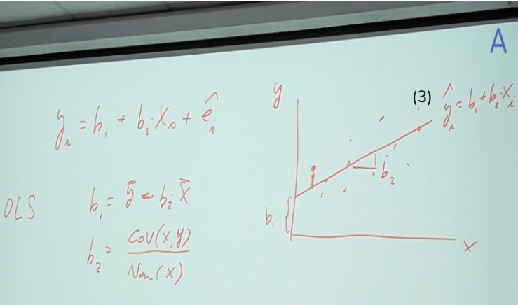
圖: a (下面還有公式)
複習Assumption of Least squaqre (注意-2,3-更正上週說法)
1.linear relationship
2.E(ei | xi) =0 has two implications(兩層意義): E(ei)=0 and
Cov(xi,ei|xi)=0
(見📌講義p.9 2.1 )
3.var(ei|xi) =δ^2
4.Cov(ei,ej | xi) =0
5.xi is nonstochastic (非隨機的)
6.ei~ N(0,δ^2) -> ( δs2= Σ(ei-ebar)^2 / n = Σ(ei)^2 /n )
δhat2= Σ(ei^ - e^bar )^2 / (n-1) = Σ(ei^) ^2 /(n-1)
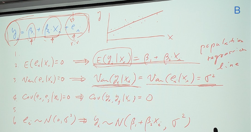
圖: B相片
2.E(ei | xi) =0 so-> and E(yi | xi) = β1 + β2 xi (=population regression line)
3.var(ei|xi)=0 so-> var(yi|xi)= var(ei|xi) =δ^2
4.Cov(ei,ej | xi) =0 so-> Cov(yi,yj | xi) =0
5.
6.ei~ N(0,δ^2) so-> yi~ N(β1+β2xi,δ^2)
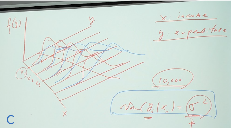
圖: c 相片 立體圖用 income/expenditure為例 (下面還有公式)
不同的x(比如xi=$1,000元)會有很多y點(expenditure)的分佈
每條x上的y 都會是normal distribution
📌講義p.8 2.2.1 All
pairs drawn from the same population are assumed to follow the same
joint pdf and are identically distributed i.i.d
(理論上: 每條y的distribution 變異數variance都一樣所以樣子都一樣)
理論如此,但實務上不會那麼剛好,所以可能像藍色線那樣分佈。
以上是Quick Review for Basic Concept
現在看講義快速過一次, 有10節 但有些節會跳過去(可回家自己慢慢看)
📌講義p.4 2.1 The
pdf f(y) describes how expenditures are distributed over the population
since Households with an income of $1000 per week would have various
food expenditure per person for a variety of reasons.
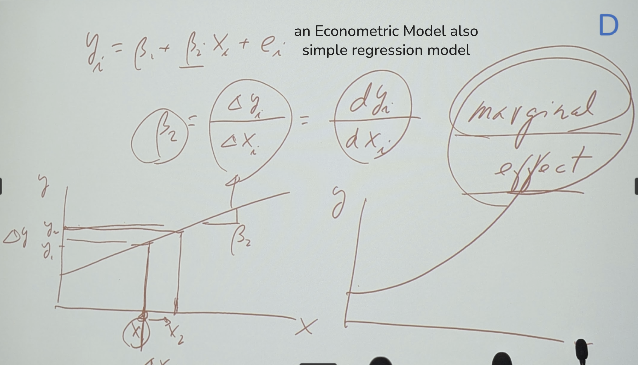
2.2 exogeneity 外生性; 複習為什麼economic model上叫做 marginal effect
(看圖d β2=dyi/dxi) will depend on your current situation, always the
same. 2.2.4 𝑣𝑎𝑟 𝑒𝑖 𝑥𝑖 = 𝜎2 This is the homoskedasticity (homo=same;
skedasticity=variance)
📌講義p.18 2.2.9
Summarizing the Assumptions 接下來p.19舉例:
想想我們怎樣找出這個yi^ 看p.21 (2.5) (2.6) 如何去fitted
regression line
which is: the Best Linear Unbiased Estimators. We call this is BLUE estimaors是一個formular, 就是說: 這個formular一旦用OLS方法可以找出b1,b2 我們就稱這個formular是BLUE。
至於為什麼?你可以去看教科書的附錄,那裡有BLUE的公式推導證明。
📘課本 p.375 8.4.1 Transforming the Model: Proportional Heteroskedasticity
看講義p.23有b1,b2的公式
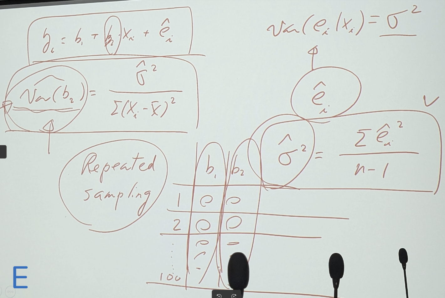
var(b2) = δhats2 / Sumation(xi-xbar)^2 and δhats2 = ehati s2 /n-1
請參考講義p.29- 2.4.3 Sampling Variation
奇怪,b2不是只有一個數字嗎,怎會有var(b2)? 這是因為 因為有Repeated
sampling的關係 見相片F 有表格 b1 b2 1,2,3….100
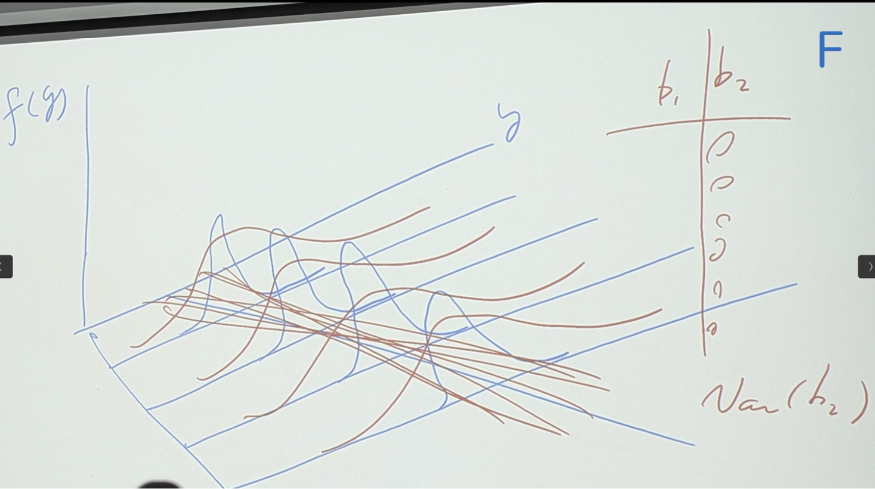
會何需要用這想法?你就要回去看立體圖 相片(圖: c) 因為x1…xi 每個x會有很多不同的yi 這樣很多linear line會有不同的var(b2) 看見相片f
(跟c很像的立體圖 但有var(b2)公式) 當你作了很多Repeated sampling 後, var(b2)可看出是寬或窄 你的母體怎樣 sampling就會長怎樣 你只要看Repeated
sampling的var(b2)就可看出分佈是寬或窄
b2最重要 他就是marginal effect 請記住公式(2.15)
Exercise food.wf1 重跑Eviews 展示: income +ctl expenditure > open as group > view -ploat sactter + fited line= regression line Quick: estimate equation : expenditure c income > method default to LS -確定 > 解讀result: C INCOME 你可以看到b2 就是income的 SD 他的square就是 var(b2)
如果你想產生y^ -> 去做Forcast (他增加一個food_expf 新的變數 focast的意思) income +ctl expenditure +cal food_expf> open as group > view -ploat sactter + fited line= regression line 就可以看到focast 的線條
income +ctl resid > open as group > view -ploat sactter 可看到residule 分佈
Residule不用管大或小,但在意是不是constant?
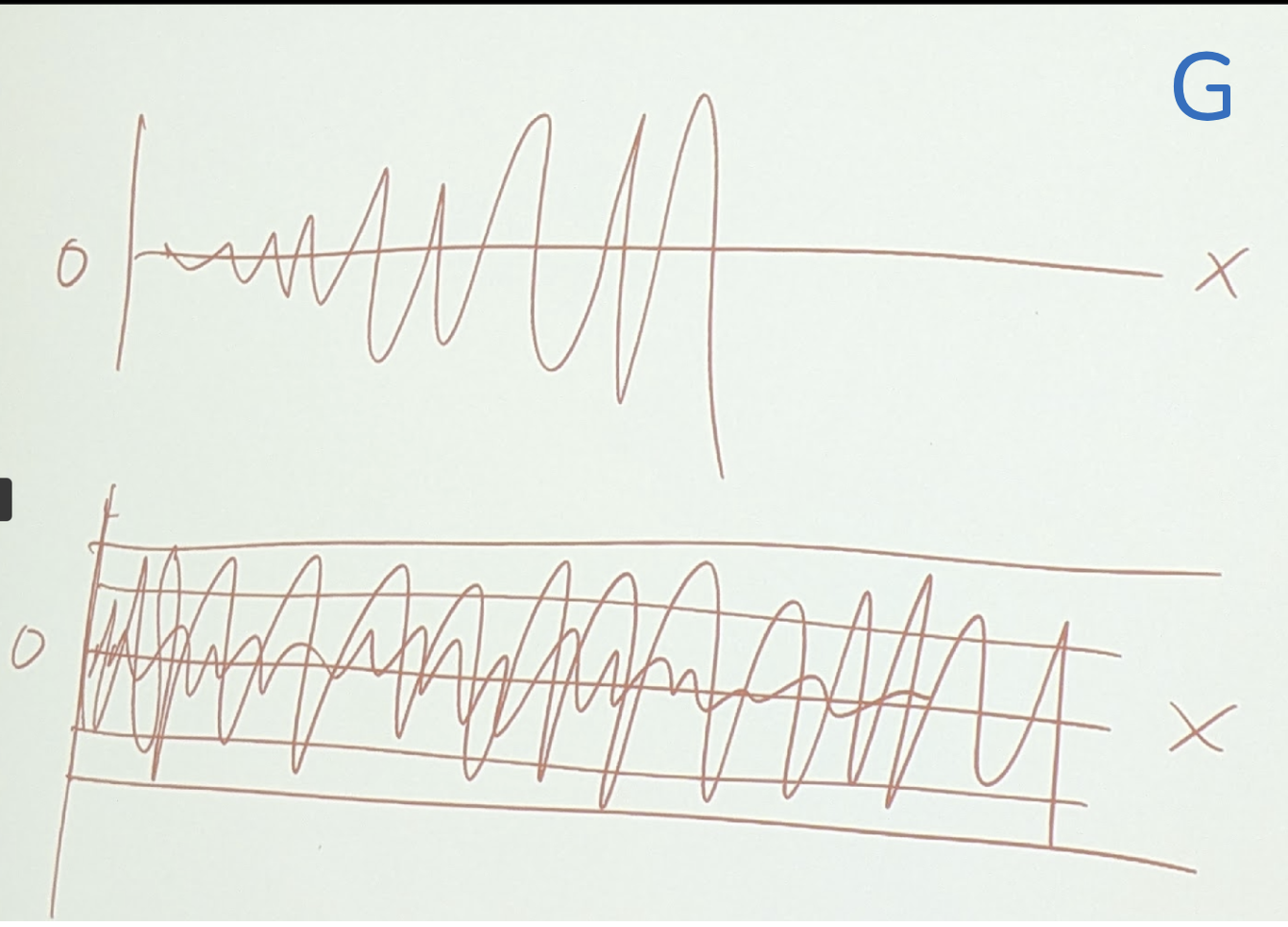
看圖G: 所謂constant就是 在一定範圍內震盪(變化),而不是越來越大或越變越小。
舉另外一例 📌講義p.47 2.2.9 Figure 2.14 A Fitted Quadratic Relationship
因為原先x,y的關係是Quadratic Relationship而非Linear Relationship,怎麼辦呢?有兩種方法可以嘗試: 1.是把independent variable SQFT再square一次 設法把曲線變為線性關係
2.另一方法是處理dependent variable y,把y做Logarithmization,即 log y也可以
但兩種方法需要比較,看那個線型比較好? (以能和最多iPair發生關係的最好)
現在用EXAMPLE 2.6 Baton Rouge House Data 來做練習 (使用資料檔br.wf1)
- sqft + ctl price > open as group > view -graph -sactter >看起來不像learning Eviews有兩種方法可run qudratic or log equation:
- price c sqft^2 > result > forcast pricef (fitted value) 會出現變數 pricef 這是第一個model
- sqft + ctl price + ctl pricef > open as group > view -graph-sactter
- log(price) c sqft > result > forcast pricef2 (fitted value) 會出現變數 pricef2 這是第2個model
- sqft + ctl price + ctl pricef2 > open as group > view -graph-sactter -ok
將兩個圖疊起來做比較,看誰比較線性!
- sqft + ctl price + ctl pricef2 + ctl pricef > open as group > view -graph -sactter -ok
那一個比較好?請看講義p.52的討論: 2.8.5 Choosing a Functional Form
(在這個case是 (2)比較好,因為他可以掌握最多的資料)
作業:📘課本
p.93這個練習
2.11.2 Computer Exercises
The capital asset pricing model (CAPM) is an important model in the field of finance. It explains variations in the rate of return on a security as a function of the rate of return on a portfolio consisting of all publicly traded stocks, which is called the market portfolio. Generally, the rate of return on any investment is measured relative to its opportunity cost, which is the return on a risk-free asset. The resulting difference is called the risk premium, since it is the reward or punishment for making a risky investment. The CAPM says that the risk premium on security j is proportional to the risk premium on the market portfolio. That is:
rj - rf = βj ( rm - rf )
rj − r = αj + βj ( rm − r ) + ej
b. In the data file capm5 are data on the monthly returns of six firms (GE, IBM, Ford, Microsoft, Disney, and Exxon-Mobil), the rate of return on the market portfolio (MKT), and the rate of return on the risk-free asset (RISKFREE). The 180 observations cover January 1998 to December 2012. Estimate the CAPM model for each firm, and comment on their estimated beta values. Which firm appears most aggressive? Which firm appears most defensive?
c. Finance theory says that the intercept parameter αj should be zero. Does this seem correct given your estimates? For the Microsoft stock, plot the fitted regression line along with the data scatter.
d. Estimate the model for each firm under the assumption that αj = 0. Do the estimates of the beta values change much?
下週要開始第3章講 Interval Estimation and Hypothesis Testing
W06 Chp03 Interval Estimation and Hypothesis Testing
2025-10-15-Tuesday 14:00-17:00 林師模教授
課本: Principles of Econometrics, 5th Edition | Chp03 第112頁開始。
講義: Ch-03 Interval Estimation and Hypothesis Testing | Youtube Descriptive Statistics vs Inferential Statistics |
溫故知新: Quick Review of Chp.02
最重要的3個公式
(1)yi =β1 + β2 xi + ei (econometric,regression model; population regression line)
(2)yi =b1 + b2 xi + ei^ (sample estimator model; b1,b2 are estimators of β1, β2; call ei^ as residule)
(3)yi^=b1 + b2 xi (call sample regression line)
以food.wf1為例,用Eviews跑資料:
Estimation Command: LS FOOD_EXP C INCOME
Estimation Equation: FOOD_EXP = C(1) + C(2)INCOME
Substituted Coefficients: 就得到結果如下,以及下表
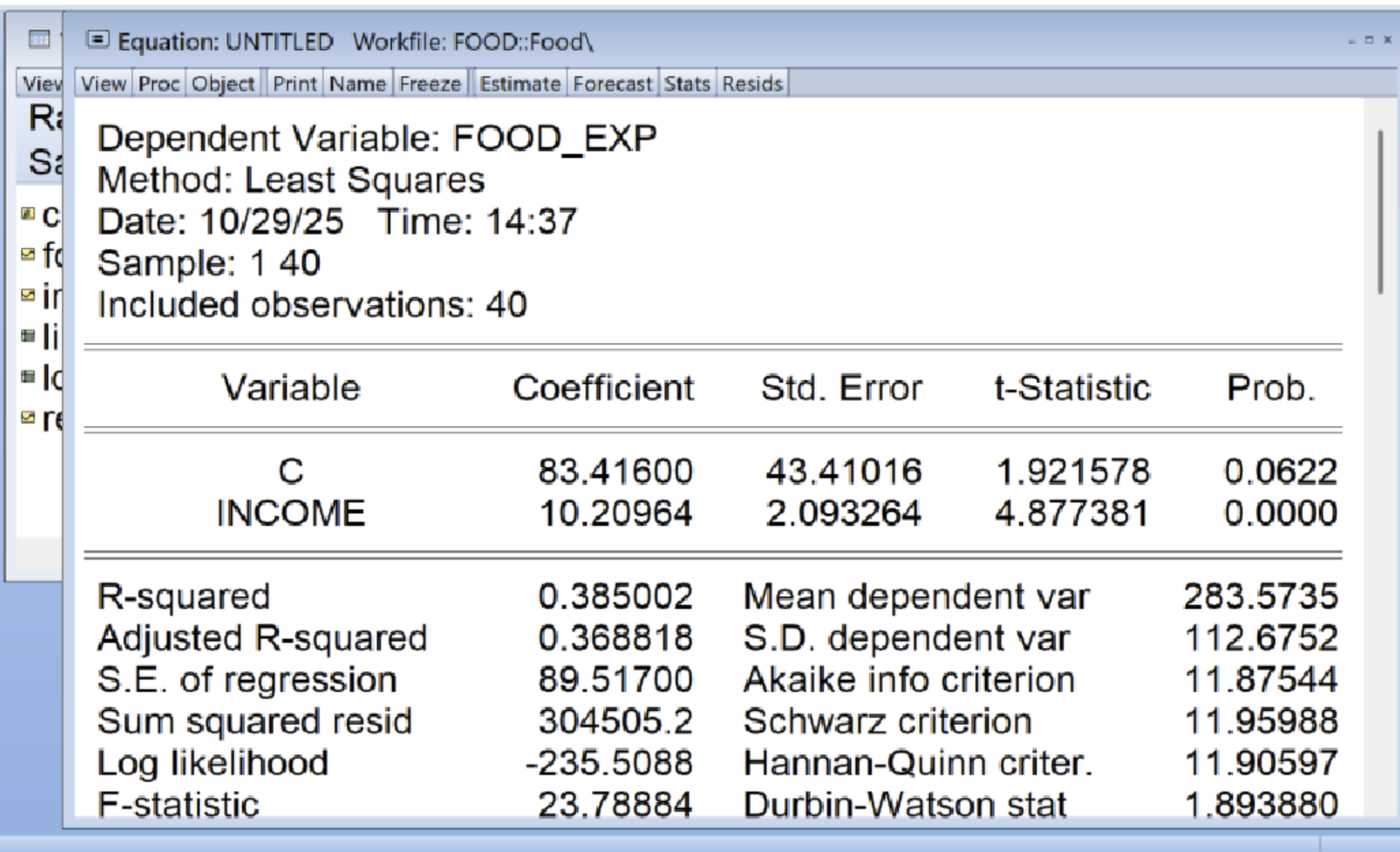
FOOD_EXP = 83.4160020208 + 10.2096429681INCOME
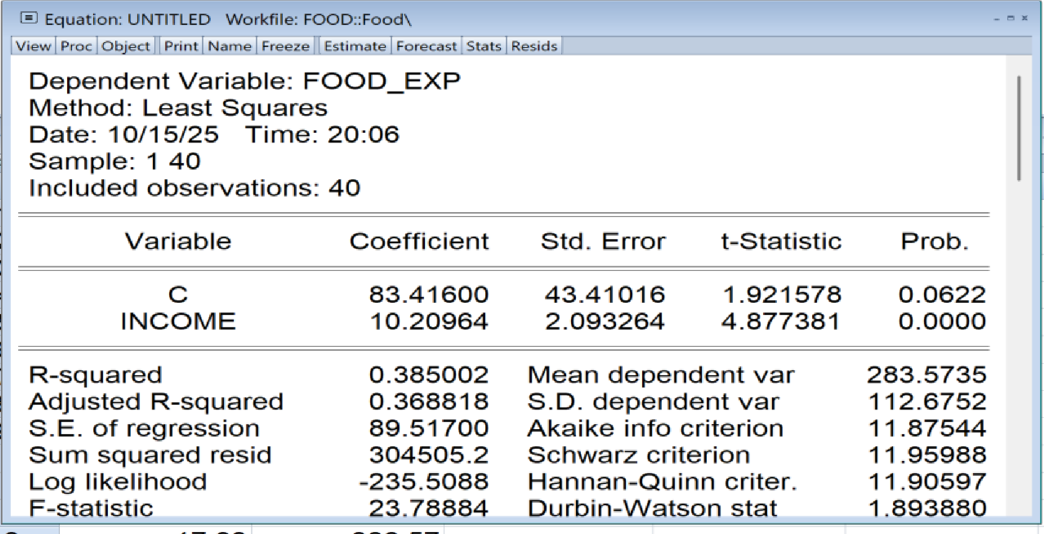
(表1)
清楚知道:
C (就是b1) 係數等於 83.41600 標準差Std.Error是 43.41016
INCOME (就是b2) 係數等於 10.20964 標準差Std.Error是 2.093264
而且(表1)表格中說:
S.E. of regression = 89.51700 (把這個squared就是 σ^2)
Sum squared resid= 304505.2
Mean dependent var =283.5735 (這就是 y bar)
S.D. dependent var =112.6752
現在我們要來研究 var(β2):請看
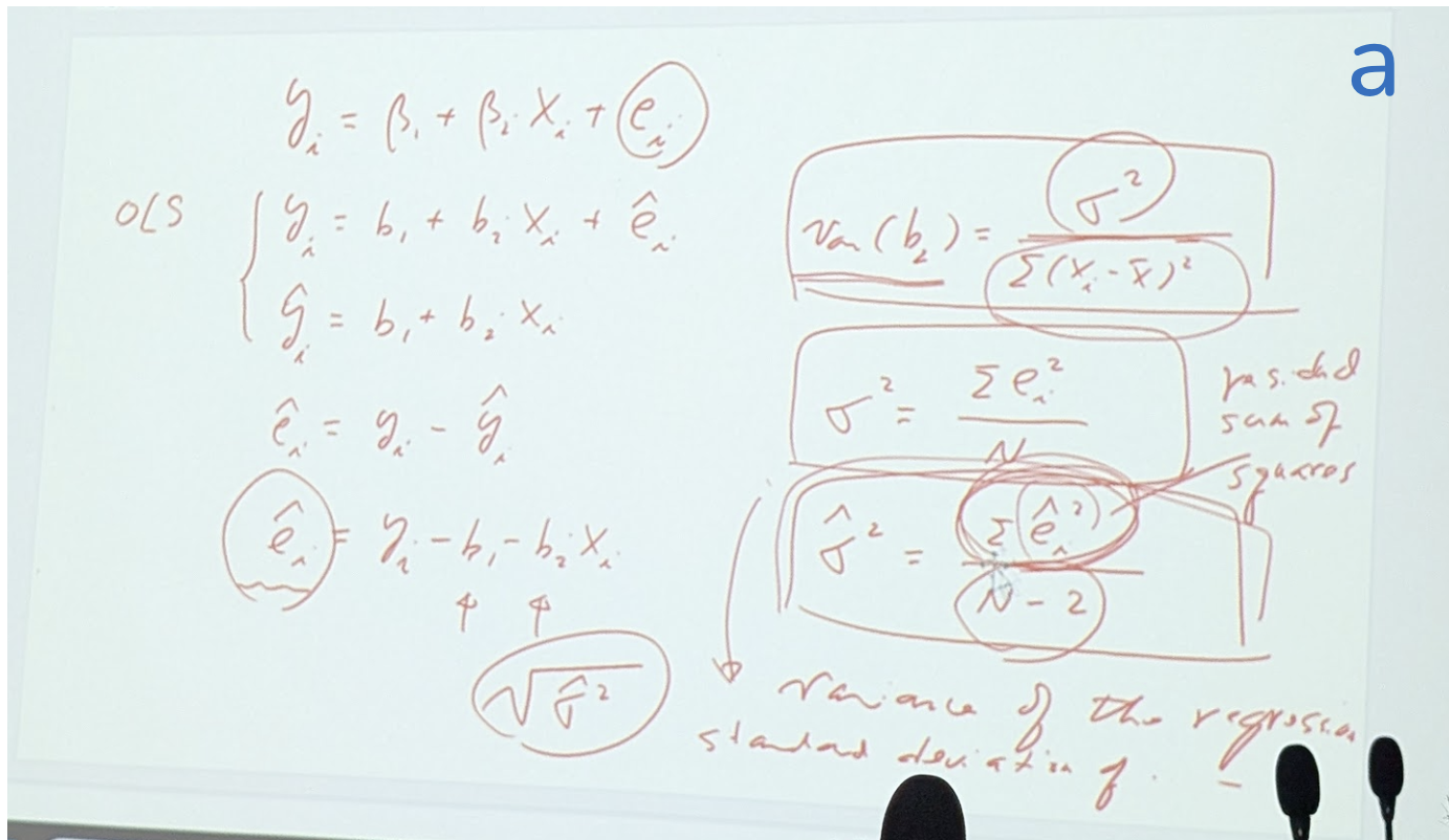
(圖a)
因為 var(β2)= σ2 /
Σ(xi-xibar)2
那首先就要先弄清楚σ2
和Σ(xi-xibar)2 的值。
1.σ2: Sum squared residule的公式是 σ2 =
Σ ei2 / N 但因沒有population只有sample,
所以改用 σ^2 = Σ ei^2 / N-2
(少掉b1,b2兩個)
因為Eviews已算出 Sum squared residule =304505.2 這就是Σ
ei^2,
而將這個Σ ei^2開根號(再除以38)就是S.E. of
regression = 89.51700 這就是σ^2
(反之: (89.51700)2 * 38= 304505.144982 =Sum squared
residule)
因ei^ = yi -b1 -b2 xi (失去b1,b2兩個的df)
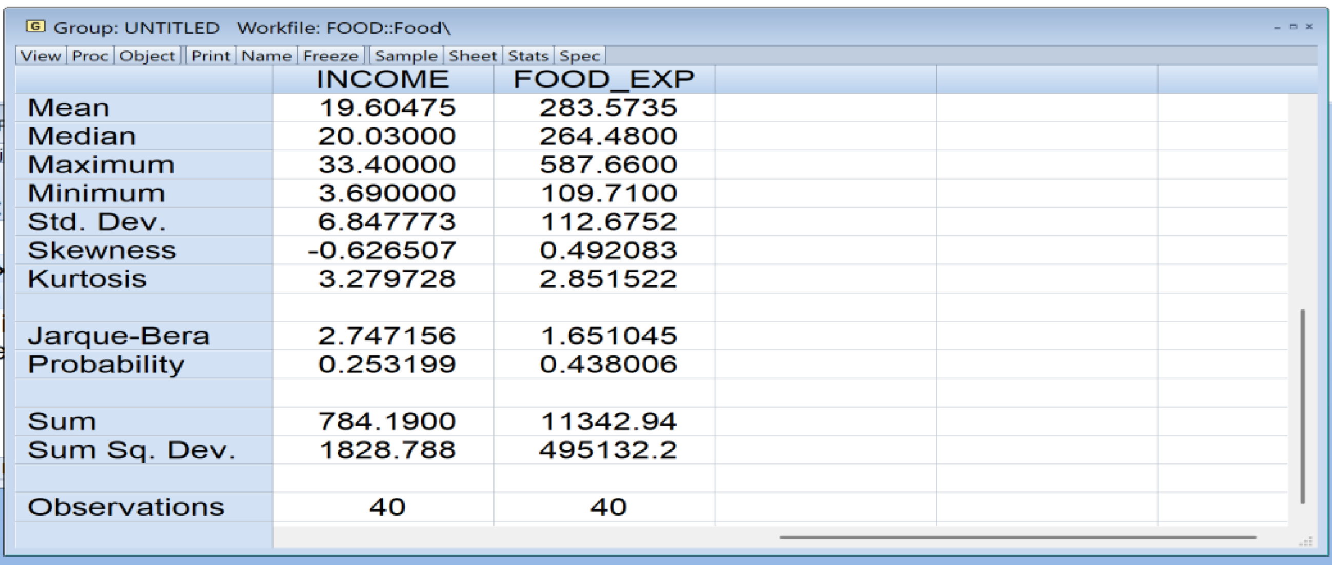
(表2)
2. Σ(xi-xibar)2:
因為 var(x) = Σ(xi-xibar)2 / N-1 在Eviews選變數[income+Ctl
food_expd]->Open with group->view->Discriptive Stats->Common
Sample就會出現 (表2)可看到:
Std. Dev. of INCOME 也就是 x 的 Std. Dev.= 6.847773
Std. Dev. of FOOD_EXP 也就是 y 的 Std. Dev.= 112.6752
公式 var(x) = Σ(xi - xi bar)2 / N-1
所以Σ(xi - xi bar)2 = (Std. Dev of x)2 *
(N-1) = 6.8477736.84777339 =1828.788
現在我們會算也會看這些關係了,可以知道各個 value of regression。
now we interested in var(b2) let’s move on Chp.03
開始講第3章:
Interval Estimation:
b1 and b2 we call estimators, when get value of b1 and b2 so call
estimate.
they are called “point estimate” 點估計; empericaly some time we might
not just interested just one point, instead, interested in a range. an
interval.
那麼range怎樣找出來呢?
idea is “how can we get range” how to establish?
(1) yi = β1 + β2 xii +
ei (call population regression line)
(2) yi = b1 + b2 xi +
ei^ (sample: estimator model)
用Z公式來standardize b2
Z=b2 -β2 /Se(b2) = (StdE(b2)
請參考前面的 var(b2) 公式) StdE(b2)=se=standard error
請照著講義p.4-5 的說明展開程式,就可找出做interval的正確方法。
先standardize b2在決定confidence value-找出z value
再用公式算出interval
slightly different from Z to t, because we do not know σ only know
σ^
注意: 因為沒辦法用 sigama square 需要換成 sigama hat square 所以Z
distribution 要換成 t distribution
注意p.7 的 (3.2)公式 的 根號中的σ square 應該改為 σ hate square
才對。
注意t table查表 時須注意正確的degree of freedom.
(課本863頁TABLE D.2 Percentiles of the t-distribution查95%-1.685/df38
如果到了∞ 也是1.96和Z一樣)
- p.862-Z表TABLE D.1是查: Cumulative Probabilities for the Standard
Normal Distribution (z) = P(Z ≤ z)
注意: p.10 tc 也寫錯了 應該是 bk 才對!!
回課本p.116 去看EXAMPLE 3.1 Interval Estimate for Food Expenditure
Data
老師用food.wf1跑一次Eviews來解釋interval作法:
- food_exp c food ->Std. Error
你可以用公式自己算,也可以按按Eviews就可以輕鬆算出
- view-> coeffice diagnostics-confidence interval-chose a
confidence-或3個都要或改都可以->OK就算出來了
想想這三種confidence的interval的意義。
- 看看TABLE 3.1, 3.2 分幾次 每次只取10個sample去跑 會怎樣?
A:用「Quick」: EViews>Quick>Estimate Equation
輸入equation: xom_rf c mkt_rf
備註:
xom_rf=(rj - rf) 是因變數。
c 是常數項 (αj)
mkt_rf=(rm - rf) 是自變數。
B:也可用: 工作檔視窗點選xom_rf(再Ctrl 依序) +c (若沒選也可以在下一步驟中手動添加) +mkt_rf >右鍵Open>as Equation.
彈出Equation Specification視窗,並預填公式,若需要時此時可補填入 c >OK。
得出結果後: View>Coefficient Diagnostics>Cinfidence Intervals...>OK
就會得到 0.9 0.95 0.99 三個Cinfidence Intervals的low和hight beta value.
0.315325 < MKT_RF < 0.597717
回去要詳看一次: 課本的學習參考提示與答案
接下來p.118要講3.2:
Hypothesis Testing:
- yi = β1 + β2 xi +
ei (call population regression line)
- yi = b1 + b2 xi +
ei^ (sample: estimator model)
只要有sample總是可以得到b1 b2 (比如food的結果如下)
yi = 83.41 + 10.2 xi + ei^ 但實際上不是那麼可靠!
但如果 β2=0 表示 x沒有 effect對於y
那麼10.2 一直到趨近於0 之間,到那一個點(critical point)這個effect會變得very weak?!
這就需要做test 看看 β2=0 是否成立! 看看在這個(critical point)時 是不是significant 說他們是有顯著的關系。
如果significant 就是
H0: β1=0
H1: β1≠0
H0: β2=0
H1: β2≠0
t = b2-β2 /Se(b2) ~ tα/2, N-2
α=0.05 so α/2=0.025
4.8已進入 rejection area, which is means β2≠0, it is
significantly different from 0.
because t vale is greter than critical value (超出了α 的critical
point)
這是針對單一回歸係數的檢定!
這在3.2.2有更詳細的解釋 需要去看
還有3.3.1講的是單尾的假設檢定
下週W07-從p.123的3.4 Examples of Hypothesis Tests開始講
下課了,真好。
W07 Ch-03 Interval Estimation and Hypothesis Testing
2025-10-22-Tuesday 14:00-17:00 林師模教授
課本: Principles of Econometrics, 5th Edition | Chp03 第123頁開始。
講義: Ch-03 Interval Estimation and Hypothesis Testing
期中報告
Interval estimation is a procedure for creating ranges of values, sometimes called confidence intervals, in which the unknown parameters are likely to be located.
Hypothesis tests are procedures for comparing conjectures that we might have about the regression parameters to the parameter estimates we have obtained from a sample of data.
depend very heavily on assumption SR6
SR6:
ei~ N(0,σ2) -> ( σ2= Σ(ei-ebar)2 / n = Σ(ei)2 /n )
σ^2= Σ(ei^ - e^bar )2 / (n-1) = Σ(ei^)2 /(n-1)
p.114 interval formular derivation: The statistical argument of how we go from (3.1) to (3.2) is in Appendix 3A.
p.115 [3.1.2] Obtaining Interval Estimates
(3.4) P(−tc ≤ t ≤ tc) = 1 − α
P[−t(0.975, N−2) ≤ t ≤ t(0.975, N−2)] = 0.95
(3.5) P[bk +- tcse(bk)] = 1 - α
W07-從p.123的3.4 Examples of Hypothesis Tests開始講
1. Determine the null and alternative hypotheses.確定零假設和備擇假設。
2. Specify the test statistic and its distribution if the null hypothesis is true.若虛無假設成立,則指定檢定統計量及其分佈。
3. Select α and determine the rejection region.選擇α並確定拒絕域。
4. Calculate the sample value of the test statistic.計算檢定統計量的樣本值。
5. State your conclusion.陳述你的結論。
(老師的講義)
1. A null hypothesis 𝐻0
2. An alternative hypothesis 𝐻1
3. A test statistic
4. A rejection region
5. A conclusion
When testing the null hypothesis that a parameter is zero, we are asking if the estimate b2 is significantly different from zero, and the test is called a test of significance.
統計檢定程序無法證明零假設的真實性。當我們無法拒絕零假設時,假設檢定所能確定的只是資料樣本中的資訊與零假設相符。
“If a value of the test statistic is obtained that falls in a region
of low probability, then it is unlikely that the test statistic has the
assumed distribution, and thus, it is unlikely that the null hypothesis
is true.”
“如果獲得的檢定統計量的值落在低機率區域,則檢定統計量不太可能具有假定的分佈,因此,零假設不太可能為真。”
” If the alternative hypothesis is true, then values of the test
statistic will tend to be unusually large or unusually small. The terms
“large” and “small” are determined by choosing a probability α, called
the level of significance of the test, which provides a meaning for “an
unlikely event.” The level of significance of the test α is usually
chosen to be 0.01, 0.05, or 0.10.
” 如果備擇假設成立,則檢定統計量的值往往會異常大或異常小。
「大」和「小」這兩個術語是透過選擇一個機率α來確定的,該機率被稱為檢定的顯著性水平,它為「不太可能發生的事件」提供了含義。檢定的顯著水準α通常選擇為0.01、0.05或0.10。”
Type I error If we reject the null hypothesis when it is
true, then we commit what is called a Type I error
- we can specify the amount of Type I error we will tolerate by setting
the level of significance α
Type II error If we do not reject a null hypothesis that is
false, then we have committed a Type II error
- we cannot control or calculate the probability of this type of
error
After we have estimator, somtimes we needs to know whethere there is
meaning of the parameters: coefficent-b2 (or b1)
whethere we can use the estimat LINE to represent the estimation?
we needs to TEST
set H0: β2=0
H1: β2 != 0
where the normaly distribution of be β2 : we use t-test to see if the average is 0 or not?
p.123 run Eviews [EXAMPLE 3.2 Right-Tail Test of Significance] 用 food.wf1
equation: food_exp c income
(表1)
但如何嚴謹的推斷、證實這個假設呢(即b2>0)?我們可以做一個
Null Hypothesis(虛無假設)H0:β2 = 0。
再設一個對立假設H1:β2 > 0。
如果我們拒絕了零假設(虛無假設)H0,我們可以直接得出結論:β2 為正,並且只有很小的機率(α)我們犯了錯誤。 此假設檢驗的步驟如下:
1.設定H0,兩個假設H1。
2.指定檢定統計量及其分佈。(是抽樣,所以用t分佈。
而因為設若null hypothesis H0:βk=c為真。那麼這公式就推導為:
(3.7) 統計量 t=(bk-C) / se(bk) ~t(N-2)
而目前根據H0的設定,c=0 因此,計量 t= bk / se(bk) ~t(N-2)
4.經Eviews計算我們得到b2=10.21和se(b2)=2.09所以, t=b2 / se(b2) = 10.21/2.09 =4.88
5.由於 t = 4.88 > 1.686,我們拒絕虛無假設 β2 = 0,並接受備擇假設 β2 > 0。
結論:
We reject the hypothesis that there is no relationship between income and food expenditure and conclude that there is a statistically significant positive relationship between household income and food expenditure.
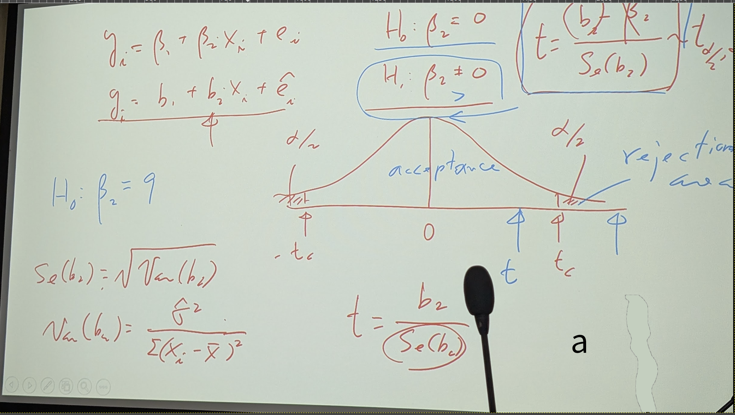
(圖a)
關於這P-value: 注意相片b "P-value"就是藍色部份 (可以拿p vs. α) 比如這裡 p=0.03 比 α(alfa) 0.05還要小
所以已經進入rejection region了,所以要reject H0.
所你也可以看t-Statistic value 也可以看 P-value (Prob)這會快多了,你不用去查t-table比對tc
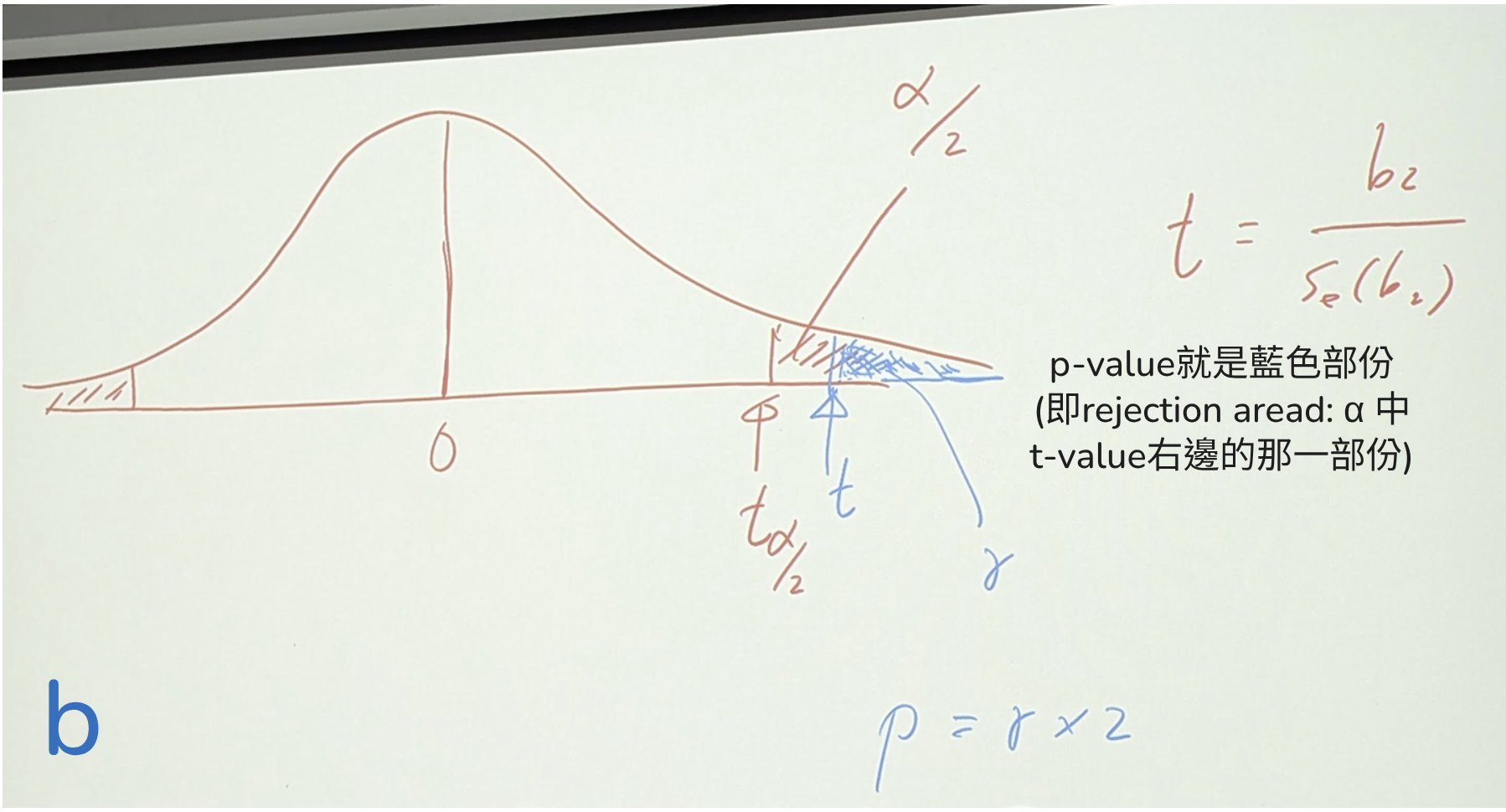
(圖b)
比如(表1)
那個C的p-value(Prob.)=0.0622,明顯就比0.05(假如是95%單尾)還大,明顯就是insignificant。Not reject。
而INCOME的p-value(Prob.)=0.0000,明顯就小於0.05甚至於比0.01,0.001都小,一看就知道是significant應該要reject Null Hyothesis。
所以說,有p-value可看時,一般就不用去查tc值來和t值比對,可以快速做出判斷。
這就是用food.wf1 看整個過程的詳細解說
★ Normally Hypothesis alternative allways one you belive, and H-null is one you want to reject!
p.124 [EXAMPLE 3.3 Right-Tail Test of an Economic Hypothesis 經濟假設的右尾檢驗]
這就是用food.wf1 看整個過程的詳細解說
現在,我們要根據收集到的40個(收入-食物支出)樣本進行推估,並提出可信服的證明給總經理做決策參考!
考量: 雖然說β2的最小平方法估計值為b2=10.21,大於5.5。但我們想要確定的是,是否有令人信服的統計證據能夠讓我們基於現有數據得出 β2>5.5的結論。這項判斷不僅基於估計值b2,還要基於其精確度(以 se(b2) 來衡量)。
2.指定檢定統計量及其分佈。
- 統計量 t=(b2-C) / se(b2) =(b2- 5.5) / se(b2) ~t(N-2) 。(若null hypothesis為真)
3.設信賴區間的 α = 0.01。
- 右尾拒絕域的臨界值是自由度為N-2=38的t分佈的第99個百分位數,即 t(0.99, 38)=2.429。如果計算出的t值≥2.429,我們將拒絕原假設。(反之: 如果t<2.429,我們將不拒絕原假設。)
4.經Eviews計算-得到b2=10.21 和 se(b2)= 2.09 所以, t=(b2-5.5) / se(b2) = (10.21-5.5)/2.09 =2.25(或 P-value=nn.nn) 。
5.因為 t = 2.25 < 2.429, 不在拒絕域中,所以不能拒絕null hypothesis H0 (即β2 ≤ 5.5)。
結論:
We are not able to conclude that the new supermarket will be profitable and will not begin construction.
(在每種現實情況下,必須根據風險評估和做出錯誤決策的後果來選擇 α,像此處就採取更嚴格的要求0.01)。
▼Eviews8.1操作法 (Wald Test 省心好辦法!)
如果是用Eviews(不必手算),這樣做
如果是用Eviews(不必手算),這樣做:
EX3.3-a: 使用food.wf1檔: Quick > Estimae Equation > food_exp c income
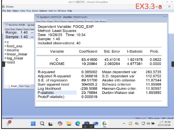
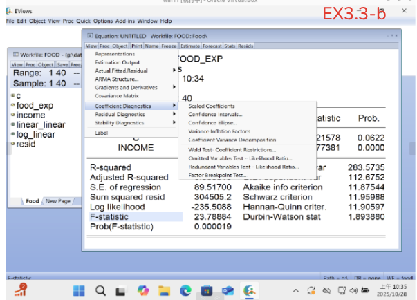
EX3.3-b: View > Coefficient Diagnostics > Wald Test-Coefficient Restirctions..
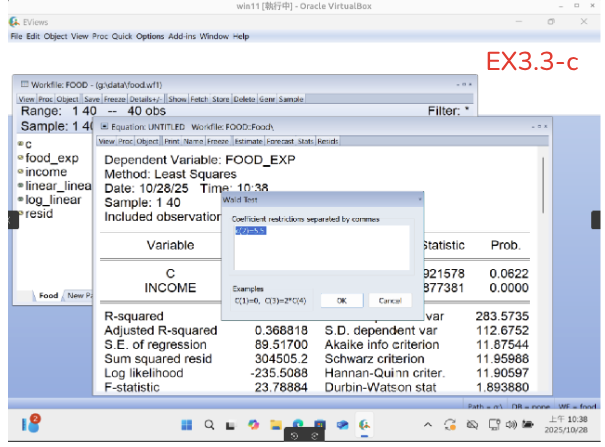
EX3.3-c: 輸入c(2)=5.5 > OK
EX3.3-d: 幫你算好t-statistic=2.249904 及p-value=0.0303 (因為要求是0.01 所以fail to reject)
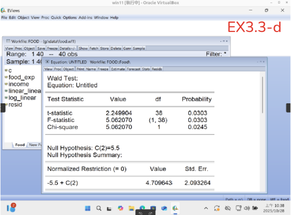
Wald-test的 c(2)其實就是 c去幫你減掉c(2)這個值 的意思。
這裡要教用view -> Cofeficcient Dignostics -> Wald-test: c(2)=5.5 -> OK
restrictions separated by commas (公式只能用 =) 請輸入
做出t-statistic 0.0303
???? 因為是2 tails所以要 0.0303/2= 0.015 比 0.01還要大 所以不能reject
*****這部份要小心 好好利用Wald-test 須搞清楚,one tail 或two
tails***會很好用!!
這兩個案例很重要,詳細做過,就了解了!!
會影響準確度有兩個因素 1.是confidence level; 2.是se(b2)-這可去看interval(分散程度)
這是簡單的例子,但其中有很多需要深思的意義。
p.125 [EXAMPLE 3.4 Left-Tail Test of an Economic Hypothesis 經濟假設的左尾檢驗]
看看他是怎樣算出結果 和如何reject null 的
為了完整起見,這裡有個(拒絕域在左尾部)的示範。我們考慮H0虛無假設 β2 ≥ 15 且備擇假設 β2 < 15。
1.Determine the null and alternative hypotheses:
設定H0: β2 ≥ 15 ,和H1: β2 < 15。
2.Specify the test statistic and its distribution if the null hypothesis is true:指定檢定統計量及其分佈:
- 統計量 t=(b2-C) / se(b2) (若null hypothesis為真)。
設信賴區間的 α = 0.05 :
- 左尾拒絕域的臨界值是自由度為N-2=38的t分佈的第5個百分位數,即 t(0.95, 38)=−1.686。如果計算出的t值≤ −1.686,我們將拒絕原假設。(反之: 如果t>−1.686,我們將不拒絕原假設。)
經Eviews計算-得知 b2=10.21 和 se(b2)= 2.09 所以,
t=(b2 - 15) / se(b2) = (10.21-15)/2.09 = -2.29
P-value=nn.nn。
結論:
由於 t = −2.29 < −1.686,我們拒絕虛無假設β2≥15,接受備擇假設β2 <15。我們得出結論,家庭每增加100美元收入,在食物上的支出不到15美元。
p.125 [EXAMPLE 3.5 Two-Tail Test of an Economic Hypothesis 經濟假設的雙尾檢驗]
注意5.Since -2.204是課本寫錯了! 應該是2.024才對 他左下的tcritical處2.024是正確的。
請看:這也是個例子 Se如過大(sample不夠多(重新取樣或或取更多sample),或是,模型只用一條簡單的回歸線是不正確的),會影響判斷結果。
某顧問認為,根據其他類似社區的情況,擬建市場附近的家庭每增加100美元收入,就會額外支出7.50美元。根據我們的經濟模型,我們可以將這個猜想表述為零假設: β2 = 7.5。如果我們想檢驗這個假設是否成立,則備擇假設是 β2 ≠ 7.5。此備擇假設並未明確 β2是大於7.5或小於7.5,但顯示它不是7.5。在這種情況下,我們就應使用雙尾檢驗,過程如下。
1.Determine the null and alternative hypotheses:
設定H0: β2 = 7.5,和H1: β2 ≠ 7.5。
2.Specify the test statistic and its distribution if the null hypothesis is true:指定檢定統計量及其分佈。
- 統計量 t=(b2-C) / se(b2) (若null hypothesis為真),所以應該是:
t=(b2 - 7.5) / se(b2)
。
設信賴區間為95% 也就是設定 α = 0.05, 那意思就是在兩個尾端各有2.5%的拒絕域。
因此兩個t-critical value分別是位在第2.5-percentile t(0.025, 38) = −2.024 和第97.5-percentile t(0.975, 38) = 2.024 的點上。
經Eviews計算-得到b2=10.21 和 se(b2)= 2.09 所以,
t=(b2 -c) / se(b2) = (10.21 -7.5) / 2.09 = 1.29 或
P-value=nn.nn。
結論:
這樣看來: –2.024 < t = 1.29 < 2.024,因此不能拒絕 H0=7.5 的虛無假設null hypothesis。 So that
our conclussion is "The sample data are consistent with the conjecture households will spend an additional $7.50 per additional $100 income on food."
也就是說:“樣本數據與以下推測一致:家庭每增加 100 美元收入就會在食品上多花費 7.50 美元。”
必須避免過度解讀這個結論。這並非從此檢定得出β2 = 7.5的結論,而只是顯示數據與該參數值並非不相容。這數據也與虛無假設H0∶β2 = 8.5(t = 0.82)或 H0∶β2 = 6.5(t = 1.77)甚至於H0∶β2 = 12.5(t = −1.09)都相容。
換句話說:假設檢定不能用來證明零假設成立,只是 不能推翻not reject。
你可能注意到了這個小技巧: 設q=100(1 − α)%
bk − tc se(bk) ≤ q ≤ bk + tc se(bk)
我們不主張使用信賴區間來檢驗假設,它們有不同的用途,但如果給定信賴區間,這個技巧就很方便。
besides, “Statistically significant” does not necessarily imply “economically significant.”
3.5 The p-Value
規則很簡單:當if p ≤ α, 就拒絕H0. 反之若 p > α, 就不能拒絕 do not reject H0 (參考上面的圖b).
p-value 其實就是: cumulative distribution function (cdf) (see Appendix B.1)
要精確計算的公式與過程是基於學生t分佈Student's t-distribution的累積機率函數Cumulative Distribution Function, CDF或其補數生存函數Survival Function, SF來進行的。
1.「精確計算」的公式在雙尾檢定Two-Tailed Test中,給定t統計量t_stat和自由度df,計算p值的通用公式為:
p-value = 2 * P(T > |tstat| with df)
其中: (以下是用到W07的作業2-b問題的內容)
|tstat|:是t統計量的絕對值,因為是雙尾檢定,我們考慮正負兩個方向的極端值。P(T > |tstat| with df):表示在自由度為df的t分佈下,隨機變數T大於|tstat|的機率,即t分佈曲線右側尾部的面積。
2 *:由於是雙尾檢定,必須將單一尾部面積乘以兩倍,以涵蓋T>3.199和T<-3.199兩側的極端機率。
個計算通常無法透過手動查表精確得到,而是依賴於統計軟體或程式庫中的數值積分。在 Python 的 SciPy 程式庫中,這個過程使用以下函數實現:Tail Area = scipy.stats.t.sf(|tstat|, df)
sf (Survival Function) 即1-CDF,它直接計算T大於tstat的機率。
程式執行方式是: htw@htwnb:~$ python3 htw_p_value_calculator.py
p.126 [EXAMPLE 3.6 Two-Tail Test of Significance 雙尾顯著性檢定]
For Econometrics, normally use this 3 tests: t-test of F-test or Chi-square-test
1.Determine the null and alternative hypotheses:
設定H0: β2 <= [??],和H1: β2 > [??]。
2.Specify the test statistic and its distribution if the null hypothesis is true:指定檢定統計量及其分佈。
- 統計量 t=(b2-C) / se(b2) (若null hypothesis為真),所以應該是:
t=(b2 - 7.5) / se(b2)
。
設信賴區間的 α = 0.01/0.05 ?。
4.Calculate the sample value of the test statistic:經Eviews計算-得到b2=ww.ww 和 se(b2)= zz.zz 所以,
t=b2 / se(b2) = ww.ww/zz.zz =[??] 或
P-value=nn.nn。
結論:
....
p.129 [3.6 Linear Combinations of Parameters]
簡單明瞭TileStatsLinear regression | hypothesis testing
t=(b1+2b2-5)/Se(b1+2b2)
Var(c1b1+c2b2) = var(λ)
covariance matrix 就是
view coe diag wal-test > hypo null 公式: c(1)+2*c(2)=5
你可以把Se 39.476 平方就是variance
var(b1)= 188 var(b2)=4.38
p.130 [EXAMPLE 3.7 Estimating Expected Food Expenditure]
這個例子就是 [3.6 Linear Combinations of Parameters]
這個沒有做什麼test
下個例子,是做出 interval estimate
p.131 [EXAMPLE 3.8 An Interval Estimate of Expected Food Expenditure]
這個計算需要先找出 se(c1b1+c2b2)
view -> Cofeficcient Dignostics -> Wald-test: hypo null 公式:
c(1)+2c(2)=5
c(1)+20c(2)=(任何number: 因為只是想找出se 就是 14.178
p.132 [EXAMPLE 3.9 Testing Expected Food Expenditure] “I expect that a household with $2,000 weekly income will spend, on average, more than $250 a week on food.” How can we use econometrics to test this conjecture?
也是view -> Cofeficcient Dignostics -> Wald-test: c(1)+20*c(2)=250
p.140 3.21 The capital asset pricing model (CAPM) is described in Exercise 2.16. Use all available observations in the data file capm5 for this exercise.
▼作業2 Asigment_2
[p.140] 3.21 The capital asset pricing model (CAPM) is described in Exercise 2.16. Use all available observations in the data file capm5 for this exercise.
a. Construct 95% interval estimates of Exxon-Mobil’s and Microsoft’s “beta.” Assume that you are a stockbroker. Explain these results to an investor who has come to you for advice.
b. Test at the 5% level of significance the hypothesis that Ford’s “beta” value is one against the alternative that it is not equal to one. What is the economic interpretation of a beta equal to one? Repeat the test and state your conclusions for General Electric’s stock and Exxon-Mobil’s stock. Clearly state the test statistic used and the rejection region for each test, and compute the p-value.
c. Test at the 5% level of significance the null hypothesis that Exxon-Mobil’s “beta” value is greater than or equal to one against the alternative that it is less than one. Clearly state the test statistic used and the rejection region for each test, and compute the p-value. What is the economic interpretation
of a beta less than one?
d. Test at the 5% level of significance the null hypothesis that Microsoft’s “beta” value is less than or equal to one against the alternative that it is greater than one. Clearly state the test statistic used and the rejection region for each test, and compute the p-value. What is the economic interpretation of a beta more than one?
e. Test at the 5% significance level, the null hypothesis that the intercept term in the CAPM model for Ford’s stock is zero, against the alternative that it is not. What do you conclude? Repeat the test and state your conclusions for General Electric’s stock and Exxon-Mobil’s stock. Clearly state the test statistic used and the rejection region for each test, and compute the p-value.
Hypothesis Testing: α = 0.05; H0: β(mkt_rf)=1 ; H1: β(mkt_rf)≠1;
equation estiamate: ford_rf c mkt_rf (by Eviews get answer:)
MKT_RF: β=1.662031 se=0.206937 t-value=8.031573 p-value=0.0000
(注意:這裡的t-Statistic=t-value 8.031573 是根據β(mkt_rf)=0 計算出來的)
t-value=(1.662031 - 1) /0.206937= 3.199 > t(0.025,178) = 2.024
且 p-value=0.0000 所以應reject H0: β(mkt_rf)=1 ,結論是 β(mkt_rf)≠1
(同樣方法再去做 General Electric’s stock and Exxon-Mobil’s stock.)
答c: Exxon-Mobil's stock (這是左尾檢定)
Hypothesis Testing: α = 0.05; H0: β(mkt_rf)≥1 ; H1: β(mkt_rf)<1;
equation estiamate: xom_rf c mkt_rf (by Eviews get answer:)
MKT_RF: β=0.456521 se=0.071550 t-value=6.380428 p-value=0.0000
(注意:這裡的t-Statistic=t-value 6.380428 是根據β(mkt_rf)=0 計算出來的)
t-value=(0.456521 - 1) /0.071550= -7.596 < t(0.95,178) = -1.686
且 p-value=0.0000 所以應reject H0: β(mkt_rf)<1 ,結論是 β(mkt_rf)<1
答d: Microsoft's stock (這是右尾檢定)
Hypothesis Testing: α = 0.05; H0: β(mkt_rf)≤1 ; H1: β(mkt_rf)>1;
equation estiamate: msft_rf c mkt_rf (by Eviews get answer:)
MKT_RF: β=1.201840 se=0.122152 t-value=9.838921 p-value=0.0000
(注意:這裡的t-Statistic=t-value 9.838921 是根據β(mkt_rf)=0 計算出來的)
t-value=(1.201840 - 1) /0.122152= 1.6523 < tc(0.95,178) = 1.6535
且 p-value= 0.050118 所以應not reject H0: β(mkt_rf)≤1 ,結論是 β(mkt_rf)≤1
答e: Ford's stock (這是右尾檢定)
Hypothesis Testing: α = 0.05; H0: α(mkt_rf)=0 ; H1: α(mkt_rf)≠0;
equation estiamate: ford_rf c mkt_rf (by Eviews get answer:)
Intercept: C=0.003779 se=0.010225 t-value=0.369564 p-value=0.7121
且 p-value=0.7121 所以應not reject H0: α(mkt_rf)=0; ,結論是α(mkt_rf)=0
A:在命令視窗: 輸入指令 genr msft_rf = msft - riskfree
genr 是generate series生成數列的縮寫。
msft_rf 是想建立的新變數名稱。
msft - riskfree 是計算公式。
執行:按下鍵盤上的 Enter 鍵。
執行後,工作檔列表Workfile window中會多出一個新的數列變數MSFT_RF出現。
下週講Chp04 Prediction, Goodness-of-Fit, and Modeling Issues
老師會跳過Prediction因為有其他工具可用(有興趣可自學),只講後面的Goodness-of-Fit,
and Modeling Issues
就是講義4.2-4.6
W08 Chp04 Prediction, Goodness-of-Fit, and Modeling Issues
2025-10-29-Tuesday 14:00-17:00 林師模教授 (換到402A教室)
課本: Principles of Econometrics, 5th Edition | Chp04 第152頁開始。
講義: Ch-04 Prediction, Goodness-of-Fit, and Modeling Issues
▼Goal of Chp04
Based on the material in this chapter, you should be able to
1.Explain how to use the simple linear regression model to predict the value of y for a given value of x.解釋如何使用簡單線性迴歸模型預測給定 x 值時 y 的值。
2.Explain, intuitively and technically, why predictions for x values further from x are less reliable.
從直覺和技術層面解釋為什麼 x 值偏離 x 值越遠,預測的可靠性越低。
3.Explain the meaning of SST, SSR, and SSE, and how they are related to R2.
解釋 SST、SSR 和 SSE 的意義,以及它們與 R2 的關係。
4.Define and explain the meaning of the coefficient of determination.
定義並解釋判定係數的涵義。
5.Explain the relationship between correlation analysis and R2.
解釋相關性分析與 R2 之間的關係。
6.Report the results of a fitted regression equation in such a way that confidence intervals and hypothesis tests for the unknown coefficients can be constructed quickly and easily.
報告擬合迴歸方程式的結果,以便能夠快速輕鬆地建立未知係數的置信區間和假設檢定。
7.Describe how estimated coefficients and other quantities from a regression equation will change when the variables are scaled. Why would you want to scale the variables?
描述迴歸方程式中估計的係數和其他量在變數縮放後會如何變化。為什麼要縮放變數?
8.Appreciate the wide range of nonlinear functions that can be estimated using a model that is linear in the parameters.
理解可以使用參數線性的模型來估計各種非線性函數。
9.Write down the equations for the log-log, log-linear, and linear-log functional forms.
寫出對數-對數、對數-線性和線性-對數函數形式的方程式。
10.Explain the difference between the slope of a functional form and the elasticity from a functional form.
解釋函數形式的斜率與函數形式的彈性之間的差異。
11.Explain how you would go about choosing a functional form and deciding that a functional form is adequate.
解釋如何選擇函數形式並確定其是否合適。
12.Explain how to test whether the equation ‘‘errors’’ are normally distributed.
解釋如何檢定方程式的「誤差」是否服從常態分佈。
13.Explain how to compute a prediction, a prediction interval, and a goodness-of-fit measure in a log-linear model.
解釋如何在對數線性模型中計算預測值、預測區間和適合度。
14.Explain alternative methods for detecting unusual, extreme, or incorrect data values.
解釋檢測異常、極端或不正確資料值的其他方法。
李柏融 卡方檢定
卡方檢定的觀念 數量資料(母數統計)-類別資料(無母數統計)>卡方主要做類別資料檢定:(觀察值-期望值)的平方/期望值=Chi square值。
Goodness-of-Fit Test ▶️適合度檢定(常態分配檢定例題),例:公正骰子,電瓶壽命。
Independent Test ▶️獨立性檢定注意,自由度是df=(r-1)(c-1),例:宗教信仰與區域性無關
Homogeneity Test ▶️齊一性檢定目的:檢定兩個或兩個以上的母體某一特性的分配是否相同或相近?注意,自由度是df=(r-1)(c-1),兩種不同肥料使發芽率是否一樣
- Examining the correlation between sample values of y and their predicted values provides a goodness-of-fit measure called R2 that describes how well our model fits the data. 檢查 y 的樣本值與其預測值之間的相關性,可以提供適合度測量(稱為 R2),該測量描述了我們的模型與資料的適合程度。 - For each observation in the sample, the difference between the predicted value of y and the actual value is a residual. Diagnostic measures constructed from the residuals allow us to check the adequacy of the functional form used in the regression analysis and give us some indication of the validity of the regression assumptions. 對於樣本中的每個觀測值,y 的預測值與實際值之間的差異就是殘差。基於殘差建構的診斷指標使我們能夠檢查迴歸分析中使用的函數形式的充分性,並在一定程度上表明迴歸假設的有效性。 - We will examine each of these ideas and concepts in turn.
p.153 [4.1 Least Squares Prediction]
p.156 [4.2 Measuring Goodness-of-Fit 配適度測量(R2) 測量擬合優度]
當我們要估計或檢定常態變數的「變異數」,時必須用到卡方分配。
(n-1)s2/σ2 服從自由度(n-1)的卡方分配,也就是 (n-1)s2/σ2 ~ χ2
χ2 = Σ(i=1,n) (Oi-Ei)2 / Ei
以上說的是卡方分配的Goodness-of-Fit; 但這裡要談的是
SST= total sum of squares
SSR= sum of squares due to the regression
SSE= sum of squares due to error
SST= SSR + SSE
R2=SSR/SST = 1-(SSE/SST)
p.159 [EXAMPLE 4.2 Goodness-of-Fit in the Food Expenditure Model]
- 請參考p.63 的[EXAMPLE 2.4a Estimates for the Food Expenditure Function]
b2 = Σ(xi-xbar)(yi-ybar)/Σ(xi-xbar)2 = SSxy / SSxx; (而b1= ybar - b2xbar)
因為: R2 = SSR/SST = 1-(SSE/SST)
這個 SSE 就是寫在 Sum squared resid (304505.2)
這個 SST 則須要拿 S.D. dependet var (112.6752) 來計算
因為公式 σ2 = Σ(y-ybar)^2 / (n-1) df = SST / (n-1) df
所以公式可代換成 SST = σ2 * (n-1)
已知
S.D. dependet var (112.6752) 這就是 σ
(n-1) = 40-1 =39 (因為n是樣本數40)
所以 SST = (112.6752)2 39 = 495130.569
因此: R2 = 1-(SSE/SST) = 1-(304505.2 / 495130.569) = 1-0.61 = 0.39 (就是這樣算出來的!)
目前只有39%的(R-squared) Goodness-fit of the line, 所以可能要換Modelshap!!
p.157 [4.2.1 Correlation Analysis]
(Ρ大寫,ρ小寫/ˈroʊ/) ρxy The correlation coefficient between x and y is defined in (B.21) -p.773ρxy = σxy / σxσy
rxy = sxy / sxsy
p.158 [4.2.2 Correlation Analysis and R2]
用Eviews怎樣算出 correlation coefficent (圖片)
選food_exp +Ctrl incomme > Open as group > View > Covarance Analysis > Correlation打勾 >OK
可以看到 food_exp和incomme 的correlation r= 0.620485
為了確認,驗算 r2 = 0.6204852 = 0.3805002 = R2 沒錯。
- Asterisks are often used to show the reader the statistically significant (i.e., significantly different from zero using a two-tail test) coefficients, with explanations in a table footnote:
* indicates significant at the 10% level
** indicates significant at the 5% level
*** indicates significant at the 1% level
寫法如下:
FOOD_EXP = 83.42 + 10.21 INCOME R<sup<2> = 0.385002
(sd) (43.41)* (2.09)***
(t) (1.92)* (4.88)***
p.160 [4.3 Modeling Issues]
p.160 [4.3.1 The Effects of Scaling the Data 數據規模的影響]
- a change in the units of measurement is called scaling the data.增減x或y 的單位,不會影響R2和 sd。
p.161 [4.3.2 Choosing a Functional Form]
- quadratic and log-linear functional forms二次和對數線性函數形式1. Power: If x is a variable, then xp means raising the variable to the power p; examples are quadratic (x2) and cubic (x3) transformations.
2. The natural logarithm: If x is a variable, then its natural logarithm is ln(x).
- Using just these two algebraic transformations, there are amazing varieties of “shapes” that we can represent, as shown in Figure 4.5.
(圖)
- elasticity change彈性變化,deviation 偏差
- 有時需要用到Quadratic 或exponatial function 可能更加better fit the regression line
所謂Quadratic 是把x squared 成為 x2; 又或許可以x不變,但是ln(y) -natural log(y)
TABLE 4.1 -Some Useful Functions, Their Derivatives, Elasticities, and Other Interpretation一些有用的函數、它們的導數、彈性及其他解釋
(回頭看p.79 的EXAMPLE 2.6 Baton Rouge House Data -這裡有計算elasticities的說明)
p.64有解釋: Elasticities還有公式和實例。
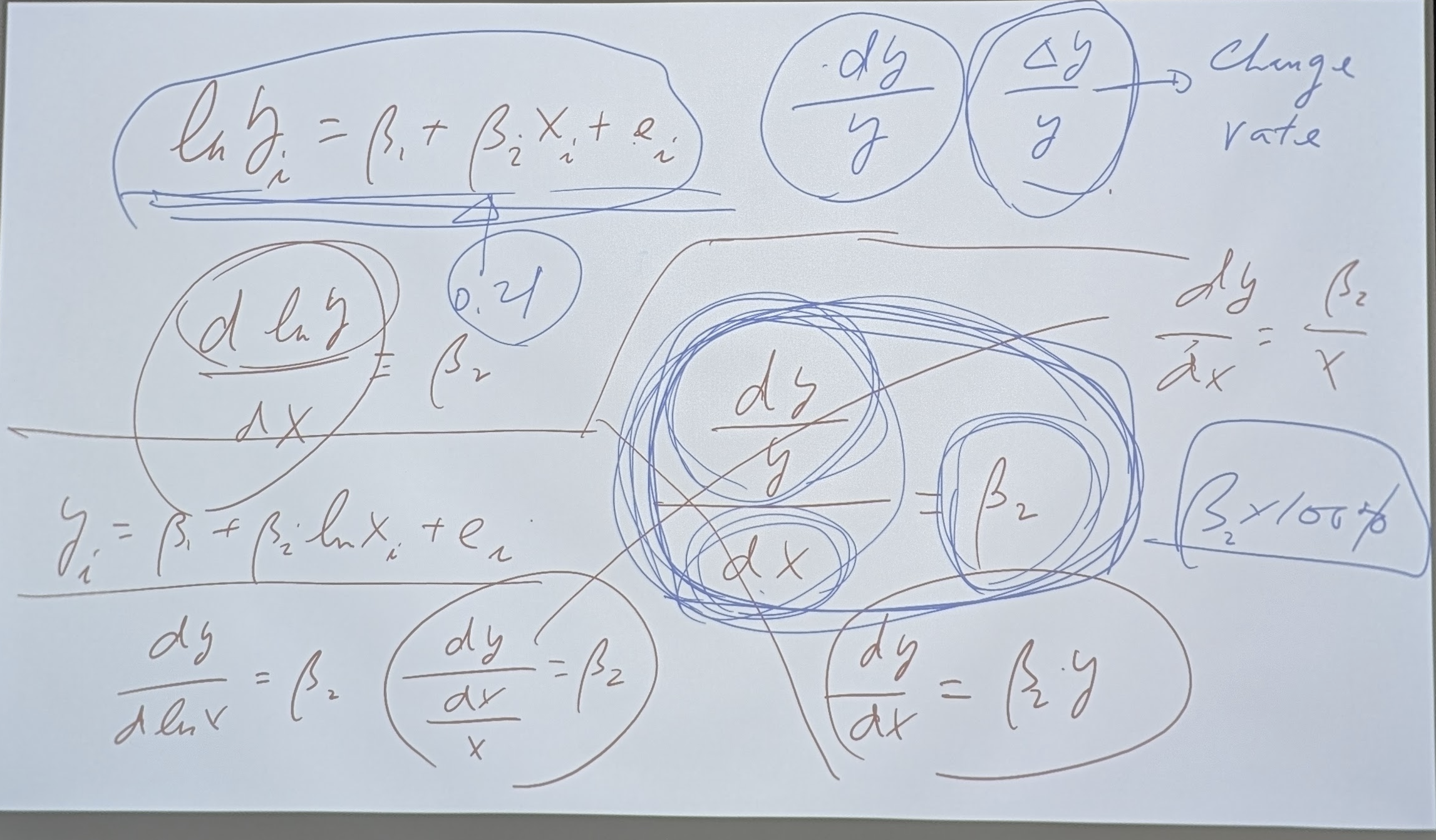
yi=β1+β2 +ei => dy/dx = beta2 = marginal effect
yi=β1+β2 x2+ei=> dy/dx = 2 beta2 x2 (如果x改為x2的話)
注意 dy/dx 的interpret, 也就是他在變動時,所代表的意義!
log > focast >
d ln(y) / d ln(x) = (dy/y) / (dx/x) = betaβ2 = 需求的價格彈性](看p.178)
p.163 [4.3.3 A Linear-Log Food Expenditure Model]
p.165 [4.3.4 Using Diagnostic Residual Plots]
p.167 [4.3.5 Are the Regression Errors Normally Distributed?]
p.169 [4.3.6 Identifying Influential Observations]
p.171 [4.4 Polynomial Models]
p.171 [4.4.1 Quadratic and Cubic Equations]
p.173 [4.5 Log-Linear Models]
p.175 [4.5.1 Prediction in the Log-Linear Model]
p.176 [4.5.2 A Generalized R2 Measure]
p.177 [4.5.3 Prediction Intervals in the Log-Linear Model]
p.177 [4.6 Log-Log Models]
p.179 [4.7 Exercises]
p.192 [Appendix]
Appendix 4A Development of a Prediction Interval 預測區間的建立Appendix 4B The Sum of Squares Decomposition 平方和分解
Appendix 4C Mean Squared Error: Estimation and Prediction 均方誤差:估計與預測
W09 --期中考--
2025-11-05-Tuesday 14:00-17:00 林師模教授
課本: Principles of Econometrics, 5th Edition |
講義: Ch-03 Interval Estimation and Hypothesis Testing
W10 --本週課目標題--
2025-11-12-Tuesday 14:00-17:00 林師模教授
W11 --本週課目標題--
2025-11-19-Tuesday 14:00-17:00 林師模教授
W12 --本週課目標題--
2025-11-26-Tuesday 14:00-17:00 林師模教授
W13 --本週課目標題--
2025-12-03-Tuesday 14:00-17:00 林師模教授
W14 --本週課目標題--
2025-12-10-Tuesday 14:00-17:00 林師模教授
W15 --本週課目標題--
2025-12-17-Tuesday 14:00-17:00 林師模教授
W16 --本週課目標題--
2025-12-24-Tuesday 14:00-17:00 林師模教授
W17 --本週課目標題--
2025-12-31-Tuesday 14:00-17:00 林師模教授
W18 --期末報告--
2026-01-07-Tuesday 14:00-17:00 林師模教授
Backup Data 其他參考資料
Book | Data Miming | Data Science for Business |
URL | Kaggle | 彭明輝教授
1.演講Youtube: 期刊論文閱讀技巧
2.演講Youtube: 研究生的核心能力 ─ 從文獻回顧到批判與創新 │Future Faculty Talk
▼1 WHAT IS INFORMATION MANAGEMENT?
WHAT IS INFORMATION MANAGEMENT?
1.ANIMATION FOR PLATONWHAT IS INFORMATION MANAGEMENT? wearesynkro 2014。2. Information Management BasicsCommunity IT Innovators 2018。
3.(IM) Information Management JuanIT 2021。有一系列lecture
4.The 5 Components of an Information System COTC A.R.C. 2015。
▼2 折疊2
折疊2
- Lorem ipsum dolor sit amet.
- Lorem ipsum dolor sit amet.